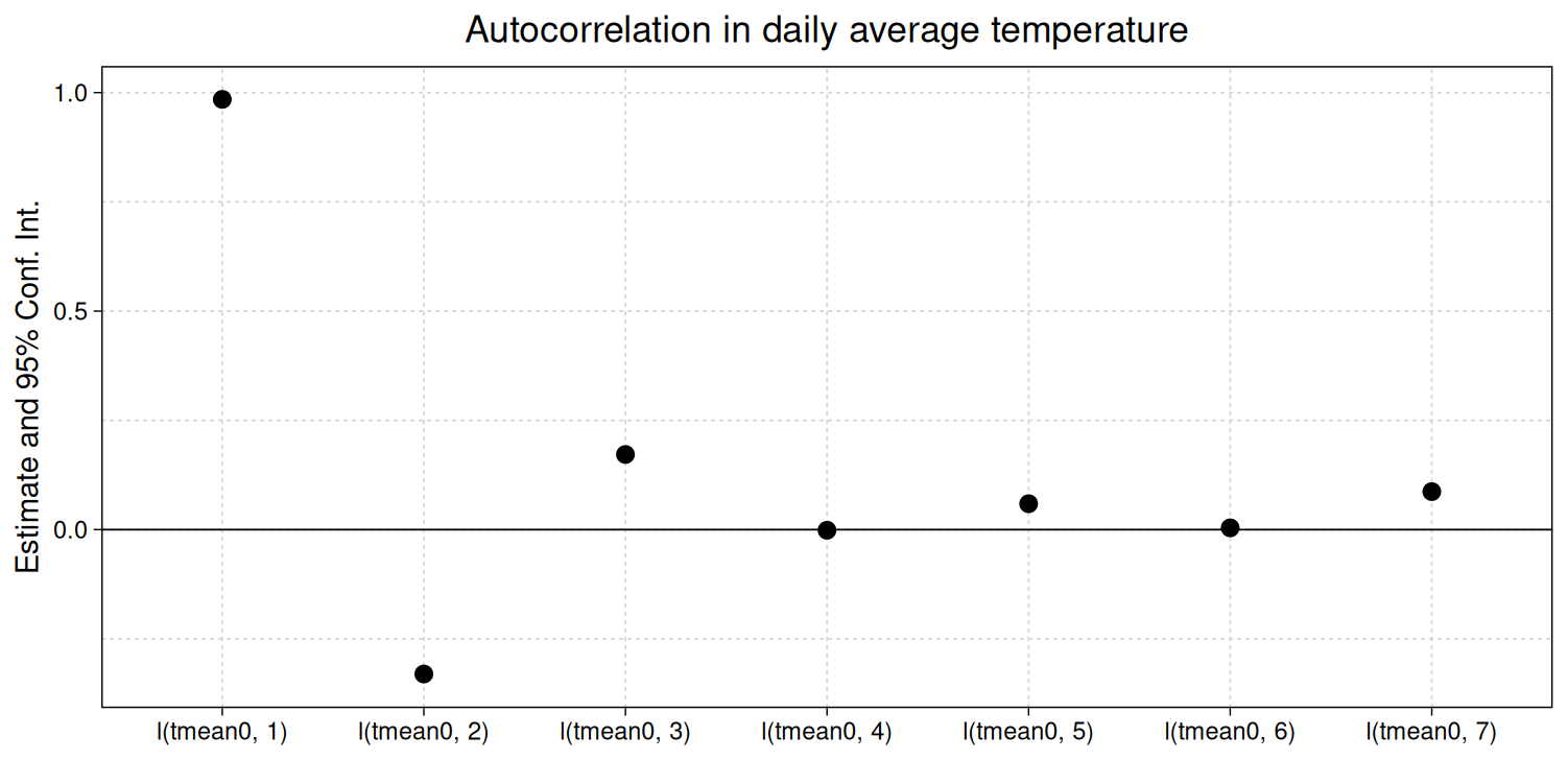
Temperature exhibits high temporal autocorrelation. Regressing daily, county average temperature in the continental U.S. on its own first lag yields a coefficient of 0.95, a t-stat of 730 (standard errors clustered at the National Weather Service County Warning Area level – a topic discussed in this post), and an R^2 of 0.9. Regressing temperature on its own first 7 lags yields the following coefficients.1
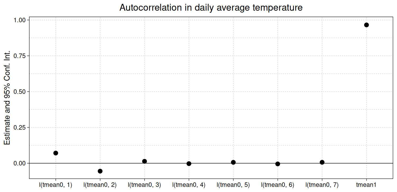
One of the econometric points I make in my weather and climate forecast papers – going back to the original draft of Improving Climate Damages – is that forecasts help identify weather effects because (among other reasons) they eliminate autocorrelation. A cool thing about weather forecasts is that they do this in a really parsimonious way. Including just a single, 1-day-ahead temperature forecast in the regression described above is enough to essentially eliminate the relationship between realized temperature and its own lag. The figure below shows regression coefficients from almost the same model but now including the 1-day-ahead forecast of daily average temperature (the variable tmean1). One can see that the coefficients for all realized temperatures move close to 0 and the forecast coefficient is near 1.
This is great! Consider all of the theorems and dynamic estimation techniques that rely on exogeneity with respect to infinite lags. Including weather forecasts makes implementation of these methods much more tractable and plausible.
But temporal autocorrelation is not the only type of autocorrelation we might be concerned with. Since reading Auffhammer, Hsiang, Schlenker, and Sobel, I have been cognizant of the extremely high spatial autocorrelation in temperature. High spatial autocorrelation is not surprising given that weather, particularly in the extratropics, are driven by large-scale convective patterns that mean neighboring locations share similar conditions. (I highly recommend staring at wind maps of the U.S.)
I was curious whether forecasts could pull off the same trick with spatial autocorrelation that they do with temporal autocorrelation. To test this, we started by basically replicating Auffhammer et al.’s Figure 2 by calculating a statistic for spatial autocorrelation (Moran’s I) for temperature and two temperature forecasts—the 6-day ahead NDFD forecast from the National Weather Service and the 10-day-ahead forecast from the ECMWF— across U.S. counties.2 The figure below shows the exceptionally high autocorrelation for all three variables across the months of the year (yellow and greenish lines at the top).
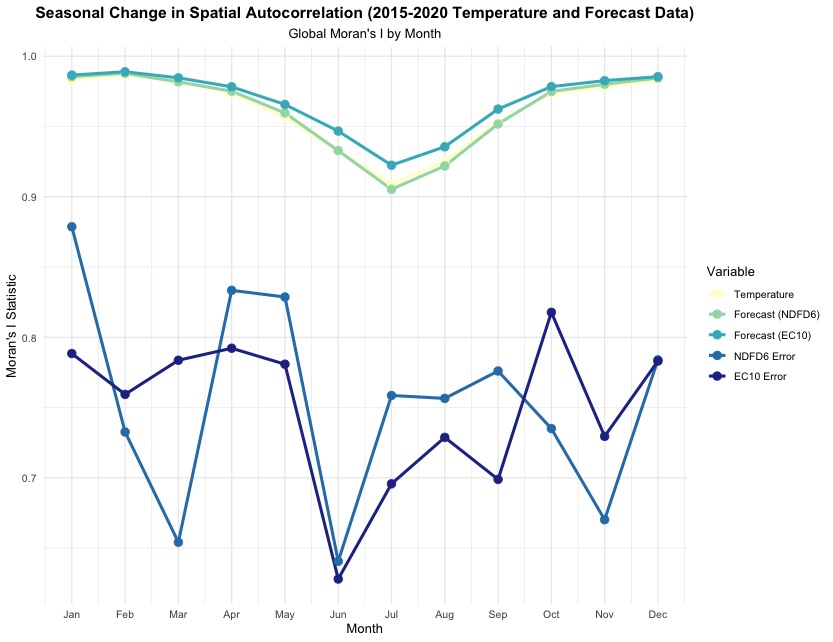
New relative to what is in Auffhammer et al., we estimated this autocorrelation for each month, and you can see that the spatial autocorrelation weakens (but remains very high) during summer months. I was surprised to see this given that hot temperatures in the U.S. tend to be more forecastable (see Figure 1 from Fatal Errors). But the dip could occur if summer months have more localized convective weather patterns such as thunderstorms? I’ll have to ask a meteorologist.
Does including forecasts eliminate this spatial autocorrelation? In short, no. The two blue lines show Moran’s I for the forecast errors from both forecasts, and though the autocorrelation is reduced, it remains well above 0.5 for even the lowest months. The spatial structure in the errors no longer shows a clear seasonal pattern, something else that I will have to think about.
Bottom line is that weather forecasts are really great at eliminating temporal autocorrelation in weather regressions but only help–rather than completely solve–issues of spatial autocorrelation.
Written with input from Max Zahrah.
Version history
2025-07-22: First version
2025-07-26: Added coefplots for time series regressions
2025-07-27: Added link to new post on CWA clustering
-
For this post, I am using data from my Fatal Errors paper, and details on the data can be found there. In brief the weather observations are from PRISM aggregated to the county level using gridcell population weights from NASA’s Gridded Population of the World. Weather forecasts are from the National Weather Service’s National Digital Forecast Database and are aggregated the same way. ↩
-
The statistic was calculated with a first-order Queen contiguity spatial weights matrix and counties with no neighbors were handled with a zero-neighbor policy. ↩